Fast Fourier Transformations part 2: The almost fourıer transformatıon

Hello again, in this post I will be talking about the underlying ideas behind the fast Fourier transformations.

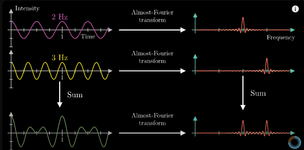
As I have mentioned in the previous post, Fourier transformations are used in waves consisting many waves of different frequencies to break down the superposition wave into its sinusoidal components. Our strategy will mainly be building a mathematical machine that treat signals with a specific frequency different than signals with other frequencies.

Let’s assume that one of the components waves exhibit the cosine function translated 1 graph above with a frequency of 2 beats per second. We inscribe the function to a circle like this(from 3Blue1Brown’s video).

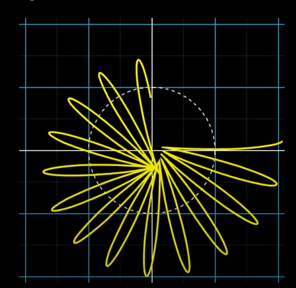
Let’s give a frequency to the vector that draws this circle. When we adjust the frequency of the vector, the shape of the circle also changes. When the frequency of the vector is the same as the frequency of our cosine function, the shape will be something like(again, from 3Blue1Brown)

Now, I propose that we imagine the shape as a full object with constant density. It also has a center of mass initially plotted at the origin. As we adjust the speed of the vector, the distance between the origin and the center of mass changes. When we plot the distance-frequency graph for the x coordinate, we will uncover the natural frequency of the sinusoidal function because when the vector frequency equals the function frequency, the distance between the two reaches a peak.

Using this property, we can identify the components of a complex wave structure. Just plug it in the model and analyze the distance graph and its peaks(not that easy, will go into more detail lol). 3Blue1Brown displayed this the best in his video

Ok time to switch things up, remember how we inscribed the graph around a circle in a 2D plane. We didn’t care about the y coordinate, but we must. So, we switch to a complex plane where the distance can be calculated by using the Euler’s formula which basically states that e^bi where b is a constant indicates the distance you would have traveled if you were to reach the coordinate. So our formula would be -e^2iftpi. And if we multiply this with our wave function which we will assume is g(x), we will get our circle-inscribed function on a complex plane. In this episode, I aimed to provide the fundamentals of the Fourier transformation and the principles. In the next post, I will approach the fat with a math and formula heavy style. Thanks for reading my post, and see you on the next ones.

Cagan out